import numpy as np
import matplotlib.pyplot as plt
import matplotlib.patches as mpatches
import math
n = np.linspace(1, 10, 300)
def norm(y):
return y / y.max()
n_factorial = norm(np.exp(np.array([math.lgamma(x + 1) for x in n])))
BG = "#0a0a14"
CARD = "#111827"
BORDER = "#1e90ff"
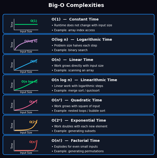
data = [
("O(1)", "Constant Time", norm(np.ones_like(n)),
"#00e676", ["Runtime does not change with input size", "Example: array index access"]),
("O(log n)", "Logarithmic Time", norm(np.log2(n)),
"#ce93d8", ["Problem size halves each step", "Example: binary search"]),
("O(n)", "Linear Time", norm(n),
"#29b6f6", ["Work grows directly with input size", "Example: scanning an array"]),
("O(n log n)", "Linearithmic Time", norm(n * np.log2(n)),
"#00e676", ["Linear work with logarithmic steps", "Example: merge sort / quicksort"]),
("O(n²)", "Quadratic Time", norm(n ** 2),
"#f06292", ["Work grows with square of input", "Example: nested loops / bubble sort"]),
("O(2ⁿ)", "Exponential Time", norm(2.0 ** n),
"#ffb74d", ["Work doubles with each new element", "Example: generating subsets"]),
("O(n!)", "Factorial Time", n_factorial,
"#ef5350", ["Explodes for even small inputs", "Example: generating permutations"]),
]
fig, axes = plt.subplots(
7, 2, figsize=(5.5, 5.5),
gridspec_kw={"width_ratios": [1, 2.4], "wspace": 0.0, "hspace": 0.0},
)
fig.patch.set_facecolor(BG)
plt.subplots_adjust(left=0.04, right=0.99, top=0.955, bottom=0.02)
for i, (label, title, y, color, bullets) in enumerate(data):
ax_bg, ax_t = axes[i]
# Transparent axes — card bg drawn via figure-level FancyBboxPatch
for ax in (ax_bg, ax_t):
ax.set_facecolor("none")
ax.set_xticks([])
ax.set_yticks([])
for spine in ax.spines.values():
spine.set_visible(False)
# Inset plot inside the left panel
ax_p = ax_bg.inset_axes([0.25, 0.21, 0.54, 0.54])
inset_bg = mpatches.FancyBboxPatch(
(0.25, 0.21), 0.54, 0.54,
boxstyle="round,pad=0,rounding_size=0.05",
linewidth=0, facecolor=CARD,
transform=ax_bg.transAxes, clip_on=True, zorder=0,
)
ax_bg.add_patch(inset_bg)
ax_p.plot(n, y, color=color, linewidth=1.8)
ax_p.set_xticks([])
ax_p.set_yticks([])
ax_p.set_xlabel("Input Size", fontsize=6, color="white", labelpad=1)
ax_p.set_ylabel("Time", fontsize=6, color="white", labelpad=1)
ax_p.set_facecolor(CARD)
ax_p.spines["top"].set_visible(False)
ax_p.spines["right"].set_visible(False)
ax_p.spines["bottom"].set_color("white")
ax_p.spines["bottom"].set_linewidth(0.8)
ax_p.spines["left"].set_color("white")
ax_p.spines["left"].set_linewidth(0.8)
ax_p.text(0.97, 0.95, label, transform=ax_p.transAxes,
fontsize=7, color=color, ha="right", va="top", fontweight="bold")
# Right text panel
ax_t.text(0.04, 0.82, f"{label} — {title}",
fontsize=9, fontweight="bold", color=color,
va="top", transform=ax_t.transAxes)
for j, bullet in enumerate(bullets):
ax_t.text(0.04, 0.50 - j * 0.23, f"• {bullet}",
fontsize=7, va="top", color="white",
transform=ax_t.transAxes)
# Draw rounded card borders in figure coordinates (rendered behind axes)
R = 0.012 # rounding radius in figure fraction
GAP = 0.003 # visual gap between adjacent card rows
for i in range(7):
ax_bg, ax_t = axes[i]
pos_l = ax_bg.get_position()
pos_r = ax_t.get_position()
rect = mpatches.FancyBboxPatch(
(pos_l.x0, pos_l.y0 + GAP),
pos_r.x1 - pos_l.x0,
pos_l.height - 2 * GAP,
boxstyle=f"round,pad=0,rounding_size={R}",
linewidth=1.2, edgecolor=BORDER, facecolor=CARD,
transform=fig.transFigure, clip_on=False, zorder=-1,
)
fig.add_artist(rect)
fig.suptitle("Big-O Complexities", fontsize=13,
fontweight="bold", color="white")
plt.show()
from IPython.display import HTML, display
display(HTML(
"Source: <a href='https://x.com/algomaster_io/status/2053806932423795081' "
"target='_blank'>7 must-know Big-O Complexities</a>"
))
# print("Source: <a href='https://x.com/algomaster_io/status/2053806932423795081' target='_blank'>7 must-know Big-O complexities</a>")